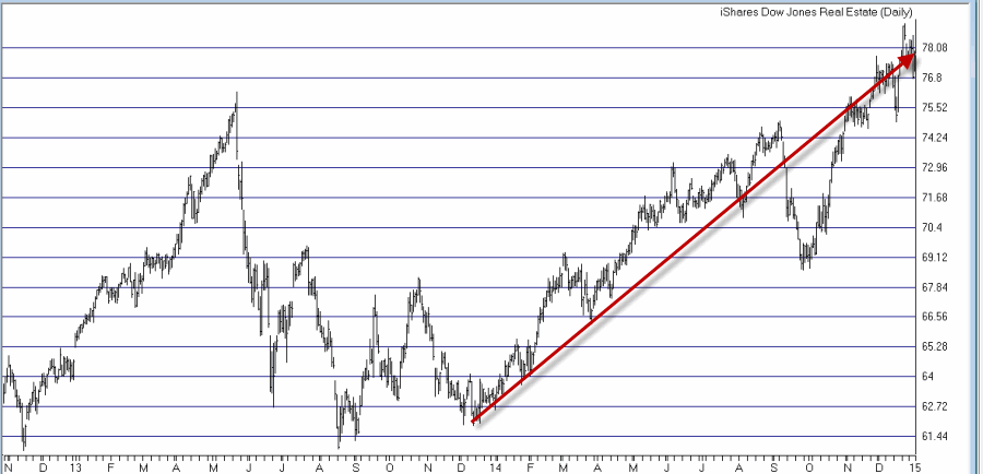
This title implies that perhaps I am talking about the fact that real estate stocks have been performing quite well of late. As you can see in Figure 1, since bottoming in December 2013, the most heavily traded real estate ETF – ticker IYR – is up over 25%. And that is a good thing.
Figure 1 – Real Estate ETF Ticker IYR (Courtesy: AIQ TradingExpert)
But the most recent rally is not what I am talking about. I am referring more to what goes on “under the hood.”
As you may know if you (WARNING: Shameless Self-Serving Plug to follow) read my book “Seasonal Stock Market Trends”, I have a “thing” for seasonality in the financial markets. And I also understand that this is also not everyone’s “cup of tea.” Depending on one’s point of view seasonal trends can either be considered to be
a) Interesting and potentially useful, OR;
b) Data curve-fitting to the nth degree
Personally I choose a), but you may choose b). And that’s OK because if we reach the point where we all trade and invest the same then there won’t be anybody left to take the other side of our trades.
The Gist of Seasonal Trends
For the record, the underlying reason that I look at seasonal trends is to attempt to find an “edge.” I would guess that 90% of traders and investors look at fundamental and/or technical analysis. I would guess that no more than 10% of traders and investors look at seasonal trends. So my rhetorical question of the day is:
If you are looking for an edge in the markets does it make sense to look:
a) Where everyone else is looking, OR;
b) Where hardly anyone else is looking?
Again, the choice is yours.
The Best Days for Real Estate
For the following illustration of using seasonal trends we will use ticker REPIX, which is the Profunds Real Estate mutual fund. For the record, this fund uses leverage of 1.5-to-1. For those who want less risk – and are willing to settle for less return – there is the Rydex real estate mutual fund (ticker RYRIX) and many real estate ETFs – with ticker IYR being the most heavily traded.
The Strategy – We will hold ticker REPIX on the following trading days each month:
*The first two trading days of the month
*Trading day’s #8, 12 and 15
*The last four trading days of the month
Obviously this particular strategy is only for traders who are “hands on” and willing to hold positions for either 1 day (in the case of trading days 8, 12 and 15) or 6 days (the four end of month days plus the two start of the next month days). Once again, this is obviously not everyone’s “cup of tea.” Still, the results are fairly compelling.
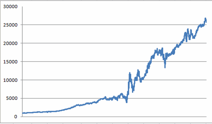
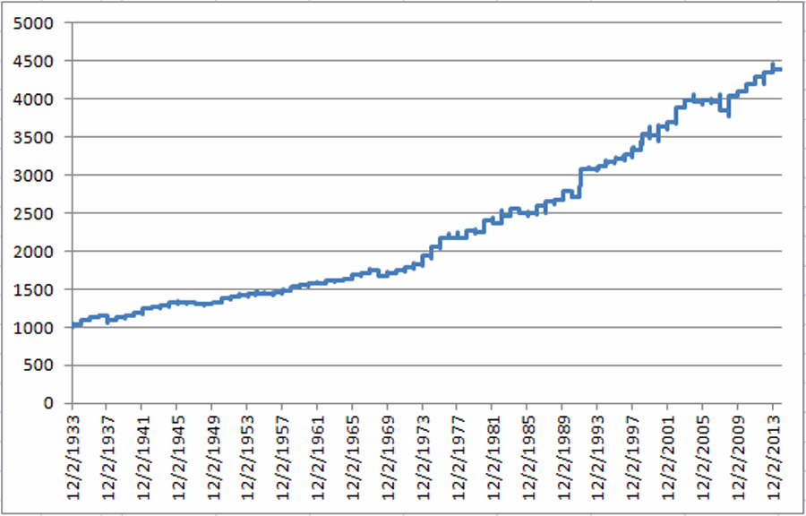
Figure 2 displays the growth of $1,000 invested in ticker REPIX only during the days listed above starting on the August 8, 2000 (when REPIX started trading).
Figure 2 – Growth of $1,000 invested in REPIX during “Best Days” (Aug 2000-present)
For the record, $1,000 invested this way grew to $25,694. Now some people will look at the return and say “hmm, that look pretty good.” Others will look at the chart itself and say “Wow, that looks way to volatile.” But looking at a set of returns in a vacuum makes it hard to really judge things.
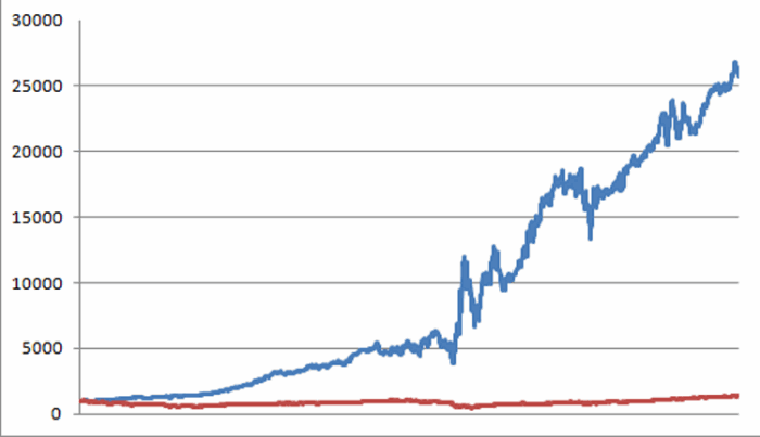
So to get a better feel for things, let’s compare the performance in Figure 2 to that of the S&P 500. In Figure 2 the blue line represent the growth of $1,000 invested in REPIX as described above while the red line represents the growth of $1,000 invested in ticker SPY on a buy-and-hold basis over the same time period.
Figure 3 – Growth of $1,000 invested in REPIX only on “Best Days” (blue line) versus SPY (red line) (Aug 2000-present)
For the record, $1,000 invested in REPIX during seasonally favorable days grew to $25,694 (+2,469%) while $1,000 invested in ticker SPY on a buy-and-hold basis grew to $1,390 (+39%).
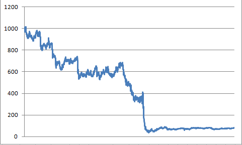
One last comparison to make is to compare the performance of REPI on “seasonally favorable” days versus “all other trading days.” Figure 4 displays the growth of $1,000 invested in REPIX only during the trading days not listed above.
Figure 4 – Growth of $1,000 invested in REPIX only on “non favorable” days (Aug 2000-present)
$1,000 invested in REPIX only on all non-favorable seasonal days actually declined in value to just $82 (-92%).
So let’s sum up the results from August 2000:
SPY: +39%
REPIX non-seasonally favorable days: -92%
REPIX seasonally favorable days: +2,469%
For the record, the difference in the relative rates of return listed above are what we “quantitative analyst types” refer to as “statistically significant.”
Summary
So is everyone going to now resolve to trade real estate stocks on certain days of each and every single month going forward? Surely not. This strategy has serious risk and volatility involved. So this is not a “hey let’s bet the ranch” type of idea. Still, a roughly 30% a year average annual return typically does involve some risk.
So most people will shy away from anything even remotely resembling what I have just described. But if you carefully reread the section above titled “The Gist of Seasonal Trends” then you may come to understand that that is exactly my point.
Jay Kaeppel
Chief Market Analyst at JayOnTheMarkets.com and AIQ TradingExpert Pro (http://www.aiq.com) client
http://jayonthemarkets.com/
Jay has published four books on futures, option and stock trading. He was Head Trader for a CTA from 1995 through 2003. As a computer programmer, he co-developed trading software that was voted “Best Option Trading System” six consecutive years by readers of Technical Analysis of Stocks and Commodities magazine. A featured speaker and instructor at live and on-line trading seminars, he has authored over 30 articles in Technical Analysis of Stocks and Commodities magazine, Active Trader magazine, Futures & Options magazine and on-line at www.Investopedia.com.